

Hi all,
I currently do an online course at MiTx, 'Underactuated Robotics' by Russ Tedrake.
'Underactuated' basically means that the robot has more degrees of freedom (DOF) than actuators. A typical example is a two-legged robot. Since it is not bolted to the ground it has extra DOF that is not directly governed by a motor, namely the toe or the heel can be considered as a pin joint around which the robot can rotate (generally referred to as 'falling').
Typically most walking robots arrange their movements such that the total of forces will always apply to a point inside the polygon formed by the two feet, resulting in a very conservative movement (for instance Asimo). The idea of this course is that if you are willing to accept to not be in full control at every moment, you can move faster and/or save energy. After all, this 'falling' is how humans walk.
When I started the course I thought that after some introduction things would become easy, because at some point the problems would become too difficult to think about, and then we would just hand them over to the computer to simulate. However, while it is true that most differential equations cannot be solved, it tuns out that there is still a lot to say about them. So the course is full of things like Lyapunov functions, Pointcaré maps, Pontraygin's Minimum Principle, Lagrange multipliers and not to forget the Hamilton-Jacobi-Bellman Equation. If you are not afraid of some Math, the course notes are here: http://people.csail.mit.edu/russt/underactuated/underactuated.html.
However, the main idea of the course is not too difficult to understand in general terms, so I will try to give an outline.
The position of a robot can be described by a number of parameters, typically the angles of the joints and the position of the robot in world coordinates. These parameters are written as one vector q. Also each of them has a speed, written as q_dot (written as a q with a dot above it). The total of q and q_dot is called the state of the robot, written as x. So basically x is a list with numbers that fully defines the state of the robot at time t.
Now the state of the robot will change, and this is a function of the current state plus the servo input. The servo input u is another vector, so it stands for a list of values, typically servo torques. The vextor x_dot describes how the state of the robot will change in the next moment. The function f is defined by the mechanics of the robot. This can be written as x_dot = f(x, u).
So in one little formula we have captured the basic scheme of every robot. Not that this formula tells a lot about any robot in particular, it just gives a common language to talk about a large class of robots.
The rest of the robot control problem can be described in similar ways. Often we know the robot in a certain state at time 0, and we want it to end in a certain state at time t. So we have x(0) = x_0 and x(T) = x_desired. And often we want to get to that goal while minimizing the total time T or for instance the total of the applied force over time.
Now the general idea of the course is that we can write all these functions down in some abstracted form and hand them over to a computer algorithm that solves it all. It's magic! There are several solvers available, some free and some commercial. What they do is not so magic in fact, in the basis they work very straightforword, they all minimize a cost function given a set of constraints. But because they have a very general use (not restricted to robotics) they are well-developed and efficient; they use a lot of tricks to speed up the process.
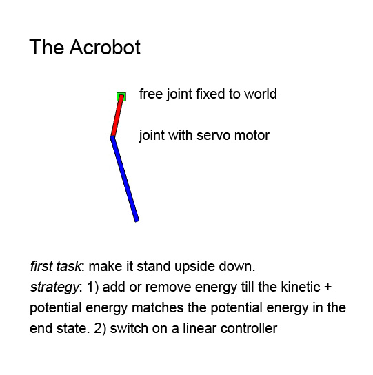
In the video the first simulations (getting the robot up-side-down) was done without a solver like this. Instead the task was to solve the problem based on mechanical insights. As you can see it does work, but barely. Maybe I can improve it, but even then there is no guarantee that the controller will always find a solution in reasonable time. In the second simulation (catching a ball) we did use a solver and you can see how it finds a very efficient solution. And when the cost function is changed, it finds quite a different solution that matches the new constraint (it finds a upper-hand approach to catch the ball at the highest possible point)
While the algorithm is pretty fast, it is not feasible to do it real-time. Even this simple example took 1 minute on my computer, for a 3 second trajectory. Also it only works for an idealized situation only, in which all parameters including the movements of the ball are known at high precision.
So the final step is to add a simple linear controller on top of the ideal curve. It requires some Math, but it can all be done when designing the controller. The end result is a controller that gets the state of the robot + ball as an input, and then performs an easy multiplication (ok, over a matrix but very straigtforward). So this can be done in real-time. Maybe my example video is not very convincing, it can handle only very small deviations, but we will learn better tools that give better results.
Also we learn how to estimate a region of attraction for the controller. This means that for a given state you can say if the controller will still work. This is a safe estimation, so it (theoretically) gives no false positive, but it can give a false negative.
The remainder of the course is about hybrid systems, that means that there is a series of movements, separated by discontinuous events. These are often contact moments with the world, for instance hitting the floor with the foot. A special case is formed by cyclic patterns like walking. And from there we learn how to extend these ideas to running, whole body movement, manipulation, swimming and flying. I can't wait!
https://www.youtube.com/watch?v=nrCMCLQcmdE