PID controller

The PID controller is a controller often used in closed loop control systems and is a controller on which three different actions act:

      1. a proportional action (P)

      2. an integral action (I)

      3. a derivative action (D)

The block diagram of a closed loop control system is as follows:

 

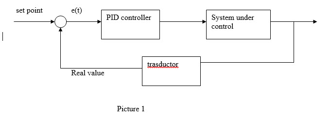
If, for example, you want to control the temperature of a room, the set-point will be the desired temperature for that room, the actual value will be the actual temperature in the room measured by a temperature probe, and e(t) will be the error of control at time instant t, ie the difference between the set-point and the actual value. Then:

            e(t) = set point – Real value

The parameters relevant to good control are:

     1. Accuracy: the actual temperature must be as close as possible to the set point

     2. Stability: fluctuations around the set-point must be small

     3. Readiness: the system should follow set-point changes as quickly as possible

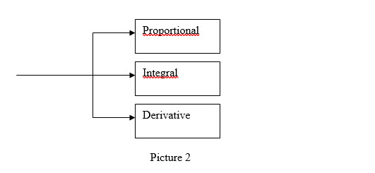
Closed loop control systems are often used in the industrial field due to the fact that they allow to act on any disturbances acting on the system under control by reducing their effects on the same, allowing also to effectively control in a short time all the physical quantities at stake on the system under control. Unlike a normal controller (for example a proportional controller), the PID controller is based not only on the variable e(t) to act on the system to be controlled, but is also based on its "history" (this is done by acting on the factor whole wheat). The structure of the PID controller is essentially a parallel between the three blocks that identify the three actions of the PID itself. Graphically we have:

 

The transfer function (input / output link) of the PID controller is as follows:

           

            Kp*e(t)+Kd*(de(t)/dt)+Ki*

where:

            Kp= Poportional costant

            Ki= Integral costant

            Kd= Derivative costant

PROPORTIONAL COSTANT:

The constant of proportionality is the constant that allows the controller to act quickly on the system under control. More precisely, if you increase Kp, the rise time decreases (ie increases the responsiveness of my system). For example, if you want to adjust the temperature of a room, and you have a set-point of 20 °C, with a room temperature of 15 °C, the control error is positive. Increasing the Kp constant also increases the product Kp*e (t) and also the output of the controller (the control variable) will be greater (this fact corresponds to a more incisive action on the part of the controller), and in this way we will reach more quickly the set-point. Increasing too much Kp, however, is likely to generate oscillation around the set-point (of overshoots). In particular, if you increase too much Kp, the action of the controller becomes too incisive and therefore there is a risk that the controlled variable of the system (in our case the room temperature) exceeds the set-point. The proportional action is characterized by a proportional time Tp.

THE DERIVATIVE COSTANT:

The constant derivative Kd instead allows to reduce the instability of the system under control and to improve the response of the same. The derivative action is based on the fact that a constant is multiplied with the derivative of the error (which can be negative or positive depending on the value of the control error). The following graphic illustrates the concept:

 

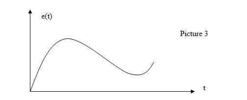
The graph in Picture 3 shows the progress of the control error over time. In particular, if e(t) increases over time it means that the difference between set-point and room temperature increases over time. So in this case the derivative of the error with respect to time is positive and this means that the product of this derivative with Kd increases (this leads to a more incisive action by the controller on the system under control). The stability of the system is linked to this action for the following aspect: through the proportional and derivative actions combined together it is possible to decrease over time and (t). When the room temperature exceeds the set-point, then e(t) becomes negative and therefore its derivative also becomes negative. At this point Kd*e (t) becomes negative, and therefore the intensity of the derivative action is subtracted from the intensity of the proportional action so that the room temperature returns to approach the desired set-point. Graphically we have:

                        Kp*e(t) + (- Kd*de(t)/dt)

 

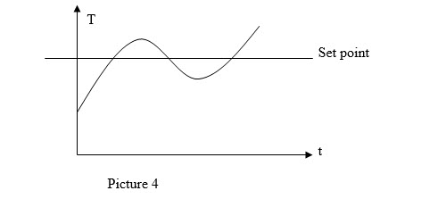
With the derivative action it is possible to make sure that the trend of the room temperature is always close enough to the set-point (oscillations of minimum amplitude). As can be seen from the graph, when the temperature falls below the set-point the derivative is positive (the control error is positive) and therefore the controller's action will increase again (Kd*de(t) / dt will return to be positive). Derivative control is characterized by a derivative time (Td). If the error signal is rapidly changing, then the output of the shunt is sufficient to bring the output power to zero.

THE INTEGRAL COSTANT:

The control error can naturally increase or decrease over time. This action, which is often used in conjunction with the proportional action, is used to indicate when the control error is to be reset. For example, if you send the error signal to an integrator whose output is added to the proportional one, the result will be that the output power increases as long as the temperature does not match the set-point. At this point the integrator output is canceled and a constant power is maintained. However, the integrator could induce fluctuations. This is avoided by the presence of proportional. The integral control is characterized by an integral time (also called reset time). It is defined as the time necessary for the output to vary from zero to its maximum in the presence of a fixed error. All three times (proportional time, integral time, and derivative time) are measured in seconds. Often Ti and Td are calculated in this way:

            Td= Kd/Kp

            Ti= Kp/Ki

Instead, as regards the three constants Kp, Ki, Kd, ​​they are expressed as a percentage (as a value, in numbers between 0 and 1).

EMPIRICAL METHOD FOR CALCULATING THE PID PARAMETERS:

There is an empirical method for calculating PID parameters.

• The control loop is closed with the PID controller, and the integral and derivative constants are set to zero. Then:

                   Ki = Kd = 0

• Starting from small values ​​of the Kp constant, a step input is inserted at the set point

• The value of Kp is gradually increased by repeating the experiment until a permanent oscillation is created around the set point.

• Based on the value of Kp and the period T corresponding to the permanent oscillation found in the previous point, the parameters of the PID are calibrated according to the following table:

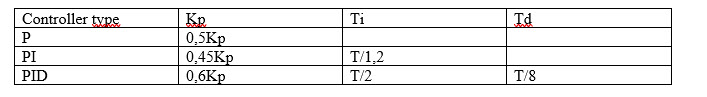
Unfortunately, this method can not always be applied because there are systems that do not generate oscillations, even with high proportional gains. The great disadvantage of this method consists in the fact that it is risky to limit the stability of the system.