

Robot Localization - So a robot really knows where it is


Robot Localization
Making a Robot know where it is

I started looking into localization for use with sandbot but there have been many other things that conspired to prevent me progressing with it. I put it here as a placeholder and will come back to this when I have more time to think about it..
Introduction
My tinkerings with robotics have lead me to the point where it should be possible to realize many of the 'cognative' functions, such as searching, mapping and localization. The aim going forward is for the robot to 'sense' the world in which it finds itself, process the sensor data and then 'move' based on the results of the processing. This sounds really obvious, but up until this stage, I have been trying to make mechanical, electrical and software domains talk to each other.
Now Sandbot has a wireless telemtry link, I am going to give it a (temporary) lobotomy. The robot will sense its environment and then transmit those readings back to the computer. The computer will perform the processing required and send commands back to the robot to move. This gives me the freedom to implement the processing (cognative) logic in a high level language on a platform that is less constrained by memory than the robot itself. In effect, the robot will become a mobile client and the computer will behave like the controlling server.
The main software loop on the robot will therefore reduce down to something like this:
  while (true) {
    transmitData(readSensors());
    move(receiveCommand());
  }
Going forward the robot itself it could have a lot of low-level intelligence to ensure it moves as accurrately as it can based on a received command. This may involve odometry and PID control although for now, it is an open-loop system. However, my focus is going to shift to the 'server' to realize some of the high-level functions.
Cognative Functions
There are several areas I would like to explore, the three main areas being:
- Searching and Exploration Techniques
- Map Building
- Localization to a map
- Combinations of the above (eg SLAM)
Once we have a map and the robot knows where it is on that map, there are several searching techniques that could be employed. A vacuum cleaner robot that knows where it has already cleaned would be infinitely better than having one that randomly stumbles around and keeps cleaning the same piece of carpet.
Building up a map in memory so the robot knows where it has been is an interesting and difficult problem. I have read about reinforcement learning and hope to use this to help with map generation. However, it is difficult to build up a map without the robot knowing where it is in the first place.
Localization involves the robot, being given a map and then trying to identify where it is on that map. This fits well with my sense-process-move architecture so this is the area I will investigate first.
Localization Prerequisites
In order to do some localization experiments, we need a map of the robot's world to work with. To make life easier for myself, the world will be made into a 2-dimensional grid where each grid square is the size of the robot footprint. This is a fairly coarse way to subdivide the problem but I need to start somewhere. If things work out, the grid may be subdivided further to give greater accurracy or even move to a non-discrete world. However, I think that the errors generated during sensing and moving will probably dwarf the granularity of the grid and I need to start somewhere.
I would like the robot to localize just using its sensors. This means no external beacons to align with and no odometery. A may need to add odometry later but humans don't navigate by counting footsteps and I don't think a robot should do either. Obviously it helps, but initially, I'll try and just use sensor data.
Initial Assumptions
The ultrasonic sensor can measure distances up to several metres. Initially, to make the problem easier to program, I will dumb down the sensor reading to be binary. Something is adjacent to the robot or it is not. I have found the ultrasonic distance sensors to be pretty accurate (more so than the IR sensors), and initially I will make the assumption that the sensor values are always correct. Later on, it should be possible to add some kind of error calculation in, but not just now.
Robot movement is more fraught with error than sensor measurements are. The robot could be commanded to move forward and it hits a wall and does not move at all. Likewise, it could be asked to turn left by 90 degrees and it only move 20 degrees. Initially, I make the assumption that the robot can move one grid square at a time and movements are always correct. I think this will need to change pretty rapidly but I'm walking, and not up and running just yet.
So, assuming the 'robot-world' is a bounded 10x10 grid and the robot can use its distance sensor to know if the adjacent grid squares are 'free' or blocked, lets investigate the 'sense' part of the problem before moving onto the 'movement' part of the sense-move cycle.
Sensing Only
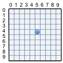
| When the robot is placed randomly somewhere in the centre of the grid, it has no idea of where it is by sensor measurements alone (all adjacent grids are free). It could therefore be in any one of 64 possible locations (all the squares not adjacent to the edges). |
| If the robot is placed in the top right hand corner (0,9), it detects a wall in front and a wall to the right. This can only happen in 4 places on the grid so the robot can be in one of 4 locations (0,0), (0,9),(9,0),(9,9). Without any further input, the robot cannot localize any better, but it is a lot more informed than the previous example. |
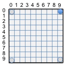
| Now lets add a compass sensor to the robot and align the grid so it is facing magnetic north. Now when the robot is in the top right-hand-corner (0,9), it sees a wall to the north and a wall to the east. There is only one square in the whole grid where this is true, so the robot is now localized and knows exactly where it is. I believe the robot need to at least know its own bearing so a distance sensor and compass should be enough for basic localization. |

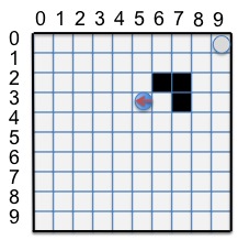
| If the robot is now equipped with a compass as well as a distance sensor, we again fall foul if there is another obstacle on the grid that looks like the top right hand corner. To the robot, grid (0,9) and (3,6) look identical. So in this case the robot could be in either of two locations. |

The above discussion shows that knowing the bearing of robot can help with localization using sensors alone. However, in the last case, although we had narrowed the localization space down to two grid squares, we can do no better. What happens if we now try to move the robot and sense again? Given we had just narrowed down to two locations, it should be possible to distinguish the two by simply moving and re-sensing.
Sensing then Moving
| This takes the previous case where the robot knew it was either in location (0,9) or (3,6). If we move west by one square and measure again, we see no blockage to the north. This means we must have previously been in (3,6) and not (0,9) and we know we are in grid cell (3,5) - given accurate robot movement. So if we iteratively sense and move, we have a greater chance of localizing to the map rather than sensing alone. |
Stochastic Processes
Up until this point, it has been possible to intuitively work out the possible locations where the robot is based on its sensor (and latterly, with movement) information. To realize this with deterministic logic in software is going to be a non-starter with a complex map, so we need to take a stochasitic approach and calculate the likelyhood that the robot is in a certain position, based on a probability distribution of all the locations in the map. This may not give black-and-white answers but we can always use a high probability as as our best estimate (eg if the probability of being in a grid cell > 0.85, then assume we are localized). It is computationally prohibitive to calculate every single move and remember its impact (like working out every combination in a chess game). A recursive mechanism where the current state is based on the previous state only is more realistic. This is a special kind of property called a Markov Chain.
When modelling the problem in software, we will need a map of the robot world in memory, as well as a model of where the robot thinks it is in relation to the real map. These are 'belief-states', namely each state represents the robots belief as to how probable it is to be in that state. For my initial investigations, there will be a 1:1 mapping between belief-states and robot-world states. On the grid diagrams, the belief-states will be overlayed on the robot-world grid (due to the 1:1 mapping).
The Starting Point - Prior Probability
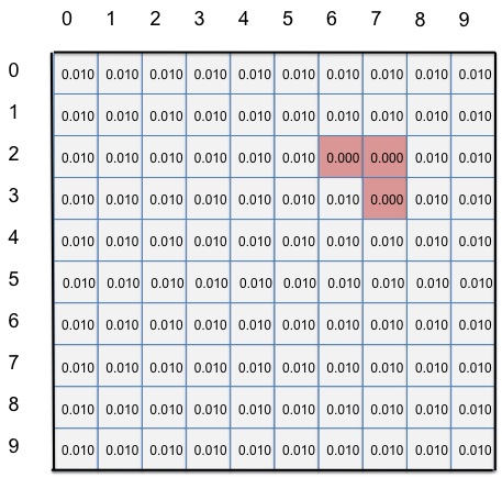
There are 100 grid cells. If three of these cells are 'blocked', that means there are 97 free locations. If the robot could be placed randomly, in any of the 97 free cells, then there is a uniform probability distribution that the robot can equally be in any of 97 locations. Assuming a zero probability of being in the 3 blocked states, this means the probability of being in any one free grid cell = 1/97 = 0.010. This is the prior probability - our starting estimate.
| This is the starting state where the robot could randomly be in any of these positions. Each belief-state therefore has a probability of 0.010. This is prior to taking any sensor readings. The only thing we can be absolutely sure of is that we are not in states (2,6), (2,7) or (3,7) as the zero probability means we can never go there. |
So what now? If we take sensor readings, how can we use this to refine our belief states? This is where Bayes Theorem comes to the rescue. Bayes theorem can be stated:
P(A | B) = (P(B | A) * P(A))/P(B)
What this is saying is we can calculate the probability of A, given B if we know the probability of B given A. This is amazingly useful as we can turn a probability around. (eg instead of saying: "what is the probability of getting heads given I randomly chose a loaded coin", we instead say "what is the probability I chose a loaded coin given I got heads on a coin flip". The key is that choosing the coin randomly was non-observable, but the result of coin flip was, and from that we can deduce something about the non-observable coin selection.
All this directly applicable to robot localization. We cannot directly observe where we are to calculate the probability of our belief-state (equivalent to choosing a loaded coin from a bag at random). However, we can sense or observe obstacles (equivalent to seeing the result of the coin flip) and from these observations, we can infer our probability of being in a belief-state.
Sensing Simulation
A program was written to simulate the sensing mechanism by implementing Bayes Theorem. The robot-world map was defined so that the robot could move north, south, east or west by one square, provided the exit was not blocked.
This is the prior. I'm using integer arithmetic and probabilities are shown as a percentage, rounded down to the nearest whole number. We can see at the start that there is a 1% (probability = 0.0103) of the robot being in any square apart from the 3 blocked ones
 Prior:
1	1	1	1	1	1	1	1	1	1
1	1	1	1	1	1	1	1	1	1
1	1	1	1	1	1	0	0	1	1
1	1	1	1	1	1	1	0	1	1
1	1	1	1	1	1	1	1	1	1
1	1	1	1	1	1	1	1	1	1
1	1	1	1	1	1	1	1	1	1
1	1	1	1	1	1	1	1	1	1
1	1	1	1	1	1	1	1	1	1
1	1	1	1	1	1	1	1	1	1
Sense test 1
Starting with our prior and applying a sense of 'free to move in all 4 directions', we get the following result. We can see the probability distribution has changed so we know we are at none of the edge cells (cannot move 4 directions) and also the cells adjacent to the obstacle. The output shows 1% in the cells but this is actually a probability of 0.0185 (truncated) so our probability of being in those locations has increased.
Posterior:
0	0	0	0	0	0	0	0	0	0
0	1	1	1	1	1	0	0	1	0
0	1	1	1	1	0	0	0	0	0
0	1	1	1	1	1	0	0	0	0
0	1	1	1	1	1	1	0	1	0
0	1	1	1	1	1	1	1	1	0
0	1	1	1	1	1	1	1	1	0
0	1	1	1	1	1	1	1	1	0
0	1	1	1	1	1	1	1	1	0
0	0	0	0	0	0	0	0	0	0
Sense test 2
Lets try another sense reading. Starting with the original prior, lets assume our sensor says we can move in any direction apart from west, the west exit is blocked. Puting this into the simulation gives quite different results. We have narrowed down the possibility of localization to 10 states, just those that are blocked to the west, giving a 10% chance of being in any one of those states. Note this includes being blocked by the obstacle.
Posterior:
0	0	0	0	0	0	0	0	0	0
10	0	0	0	0	0	0	0	0	0
10	0	0	0	0	0	0	0	10	0
10	0	0	0	0	0	0	0	10	0
10	0	0	0	0	0	0	0	0	0
10	0	0	0	0	0	0	0	0	0
10	0	0	0	0	0	0	0	0	0
10	0	0	0	0	0	0	0	0	0
10	0	0	0	0	0	0	0	0	0
0	0	0	0	0	0	0	0	0	0
Sense test 3
Lets try another sense reading. Starting with the original prior, assume our sensor tells us exists are blocked to the north and east. The results tie up with the earlier intuitive reasoning, we have narrowed our belief states down to two, and have a 50% chance of being in either state.
Posterior:
0	0	0	0	0	0	0	0	0	50
0	0	0	0	0	0	0	0	0	0
0	0	0	0	0	0	0	0	0	0
0	0	0	0	0	0	50	0	0	0
0	0	0	0	0	0	0	0	0	0
0	0	0	0	0	0	0	0	0	0
0	0	0	0	0	0	0	0	0	0
0	0	0	0	0	0	0	0	0	0
0	0	0	0	0	0	0	0	0	0
0	0	0	0	0	0	0	0	0	0
So implementing Bayes Theorem based on sensor readings across the map does indeed produce the expected probability distribution. It helps reduce the belief states but this alone will not be sufficient to fully solve the localization problem. Earlier intuitive reasoning showed that moving the robot and then re-sensing would help minimize the number of belief states and so this was the next step.
Initially, lets assume the robot moves where we want it to, one grid cell at a time i.e. if we ask it to go north it will move one grid cell north and not go east, west or stay still. Given this assumption (and that is a big assumption), what would this do to the probability distribution? Well if the whole probability distribution moves with the robot, we could get some misleading results until we sense again. However, shifting the distribution keeps a record of the movement in the beilefs states. We are in a different position now so the sensor reading change and when we apply this to the probability distribution, we should be able to pare down the number of belief states. A repeated combination of sense-move steps should eventually lead us to a unique place on the grid and we will then be localized.
Sense and Move Test 1
Taking again, the sensor reading from senseTest1
Posterior:
0	0	0	0	0	0	0	0	0	0
10	0	0	0	0	0	0	0	0	0
10	0	0	0	0	0	0	0	10	0
10	0	0	0	0	0	0	0	10	0
10	0	0	0	0	0	0	0	0	0
10	0	0	0	0	0	0	0	0	0
10	0	0	0	0	0	0	0	0	0
10	0	0	0	0	0	0	0	0	0
10	0	0	0	0	0	0	0	0	0
0	0	0	0	0	0	0	0	0	0
Now if we apply move north, using the above distribution as our prior, then sense again (and find west is blocked), we see that two belief states have fallen away (probability -> 0) and we now have a 12% chance of being in any one of the 8 states.
Posterior:
0	0	0	0	0	0	0	0	0	0
12	0	0	0	0	0	0	0	0	0
12	0	0	0	0	0	0	0	12	0
12	0	0	0	0	0	0	0	0	0
12	0	0	0	0	0	0	0	0	0
12	0	0	0	0	0	0	0	0	0
12	0	0	0	0	0	0	0	0	0
12	0	0	0	0	0	0	0	0	0
0	0	0	0	0	0	0	0	0	0
0	0	0	0	0	0	0	0	0	0
We can continue this procedure and will eventually find we converge, provided the robot can find a unique state. For example, assume we had started in state (3,8). We have sensed and moved north once. If we move north again, in reality we should be in state (1,8). When we sense in this state, we should have no obstacles in any direction (unlike all the other belief states on the western wall, so we should localize. Here are the results of doing this:
Posterior (sense):
0	0	0	0	0	0	0	0	0	0
0	0	0	0	0	0	0	0	100	0
0	0	0	0	0	0	0	0	0	0
0	0	0	0	0	0	0	0	0	0
0	0	0	0	0	0	0	0	0	0
0	0	0	0	0	0	0	0	0	0
0	0	0	0	0	0	0	0	0	0
0	0	0	0	0	0	0	0	0	0
0	0	0	0	0	0	0	0	0	0
0	0	0	0	0	0	0	0	0	0
And we have localized.
Sense and Move Test 2
Lets try one more example, that of sensetest3. In this case, after the first sense, we had narrowed down our belief state to two (3,6) and (0,9). If we move west and then sense again, if the there is no blockage to the north, we are in state (3,5), otherwise we must be in state (0,8). Running the simulation yields:
Posterior (sense):
0	0	0	0	0	0	0	0	0	0
0	0	0	0	0	0	0	0	0	0
0	0	0	0	0	0	0	0	0	0
0	0	0	0	0	100	0	0	0	0
0	0	0	0	0	0	0	0	0	0
0	0	0	0	0	0	0	0	0	0
0	0	0	0	0	0	0	0	0	0
0	0	0	0	0	0	0	0	0	0
0	0	0	0	0	0	0	0	0	0
0	0	0	0	0	0	0	0	0	0
So the test results look very encouraging. Having a pre-defined map and some suitable distance sensors, a compass and not too many errors, then applying the sensor data to the map will go a long way to identifying where we are on the map. Moving around and re-sensing will help further narrow down he choices of where we may be and by iterating through this cycle, we should be a convergent solution.
Ultrasonic Mast
In order to screw a few variables to the floor, I decided to rework the ultrasonic range finding of my test platform. Rather than having a sensor mounted on a rotating servo, I decided to have 4 separate sensors each mounted at 90 degrees to each other. This, in combination with a direction sensor should enable me to simulate the behaviour from the test localization programs shown earlier. This is perhaps an over-simplification of the problem, buts it is a good place to start.
Pin Assignment
4 ultrasound sensors require 3 extra digital pins (as one is already used by the existing sensor). The compass sensor uses the I2C bus which uses two extra pins. This is in addition to the Tx,Rx pins plus the motor control pins already in use. However, the servo will no longer be required so total I/O count becomes:
Motor:
	2 x digital outputs
	2 x PWM outputs

4 x Ultarsonic sensors:
	4 x digital I/O

UART:
	2 x digital I/O

Compass:
	I2C bust (2 pins).
That gives a total of 12 digital pins, which should be ok with the UNO board, provided I do not fin any further library clashes.
function pin

The motor pins are determined by the motor shield I am using.
motorA PWM - pin 6
motorA dir - pin 8
motorB PWM - pin 9
motorB dir - pin 7

The UART pins are determined by the Xbee arrangement.
UART Rx - pin 0
UART Tx - pin 1

Ultrasonic fwd   - pin 2
Ultrasonic rear  - pin 4
Ultrasonic right - pin 12
Ultrasonic left  - pin 13

Compass (I2C bus) SCL - pin A5
Compass (I2C bus) SDA - pin A4
I have yet to integrate or mount a compass but at this stage I want to reserve pins for it. The above pin assigments have gone for digital I/O to leave PWM outputs if required as these can always be re-assigned to digital I/O if necessary.
Firing Multiple Ping Sensors
Unfortunately, it is not possible to fire all 4 ping sensors simultaneously as the echos from the environment can be picked up by the wrong sensor and cause erroneous results. The SRF05 data sheet specifies that 50ms is required between retriggering so it will be necessray to fire them in series with suitable delays, not ideal but if we use a 65ms delay, that means all four sensors can ping and get results in just over 0.25 second. Since the robot is no longer using a servo, I should be able to slow it down (no timer fights in software) to cater for this slower measurement phase.
Test Results
Firing multiple ping sensors in series works admirably. I used a 65ms settle time between firing each sensor and the measurements returned from each sensor did not interfere with its neighbours. The only problem I have is that the 'mast' I use is near the front of the robot so the rear-facing sensor points over the arduino stack. Wires and connectors can get in the way of the sensor which will give false readings. I could move the sensor or make the tower higher to overcome the problem. I'll not get too stressed about this and make do with best I can as it is a result of the test platform not being ideal for ever configuration, it's a compromise.
The Robot-Computer Communication Link
In order to give sandbot a lobotomy, I need to be able to talk to the robot via a stand-alone program outside the arduino environment. In this way, I can write applications to test all the algorithms I need based on the data coming from the robot. In fact, once I have the interface nailed down, it will be possible to write a test-harness to simulate the robot for fine-tuning.
The arduino IDE seemed a good place to start as it has a serial communication link with the arduino board. After poking around a little, I found an RXTXcomm.jar file was where all the serial communication action was happening. I copied this arduino library and built my own Java harness around it (with help from google). The output from the arduino multi-ping program was written to the serial monitor as normal. My first Java program was able to intercept this data and display it on the console. So we have one-way comms from the robot to a custom java program which in the basis for the transmitData(readSensors()) part of the arduino code - happy days :-)
The next task was to write arduino code and java code to communicate in the other direction, namely computer -> arduino. The arduino side of this was quite straightforward, a simple 'echo' program could easily be tested using the serial monitor, the arduino sending back whichever characters it had been sent. This functionality now needed pushing into the java code and we are nearly in business, then I should have the receiveCommand() part of the project done. Small steps I know, but it takes small steps to start a long journey.
Thanks for helping to keep our community civil!
This post is an advertisement, or vandalism. It is not useful or relevant to the current topic.
You flagged this as spam. Undo flag.Flag Post
Your post is currently under review by our moderation team. The review process usually takes up to 48 business hours.
You can track your post's status in the "My Content" section of your profile. Once approved, it will be published and visible to others.

Thank you for contributing to our community!